How to Underline in Excel?

One formatting option you can use when you want to highlight a specific text or cell is the underline option.

As the name suggests, it applies an underline below some text in a cell or the entire cell.

In this article, I will cover the different types of underlines in Excel (single, double, single accounting, double accounting) and how to apply them.

While you can apply the regular underline formatting using the ribbon, you need to open the Format Cells dialog box to apply the accounting underline format.

Let me show you how it works.

Applying Underline To Entire Cell

Below, I have a data set in which I have stored names in column A, their sales values in column B, and the total sales value in cell B7.

I want to emphasize the sales value in cell B7 by applying an underline to the value.

Here are the steps to apply underline to a cell in Excel:

1. Select the cell for which you want to apply the underline formatting.
2. Click the Home tab in the ribbon

3. Click on the Underline icon

Alternately, you can also select the cell and use the keyboard shortcut Control + U

The above steps would apply a single underline to the content of the selected cell.

If you want to apply a double underline formatting, you need to select the cell and then click on the small arrow in the Underline icon. This will show you the double underline option that you can choose.

If you change the content of the cell, the underline will automatically change to ensure that it is applied to the entire cell’s content. Also, if you change the alignment of the cell’s content, the underline will also change.

Applying Underline To Some Text in the Cell

Excel allows you to apply the underline formatting to the entire cell as well as partial content in the cell.

For example, below, I have some Store IDs in column B, and I only want to apply the underline format to the number in between the two dashes.

To do this, I first need to get into edit mode in the cell, select the part of the cell that I want to underline, and then apply the underline format using the ribbon option.

Also read: How to Split a Cell Diagonally in Excel (Insert Diagonal Line)

Applying Accounting Underline to Cells

Apart from the two Underline options that you see in the ribbon, Excel also has two more underline options:

• Single accounting underline
• Double accounting underline

Accountants usually use the accounting underlines to highlight totals and subtotals in the financial data.

Let me first show you how to apply the accounting underline, and then I will explain some nuances between these different types of underlines.

Below, I have a data set in which I want to apply the accounting underline to the total value in cell B7.

Here are the steps to do this:

1. Select the cell
2. Right-click on the selected cell and then click on the Format cells option. You can also use the keyboard shortcut Control + 1.

3. In the Format Cells dialog box that opens up, select the Font tab (if not selected already)

4. Click to open the drop-down under the Underline option

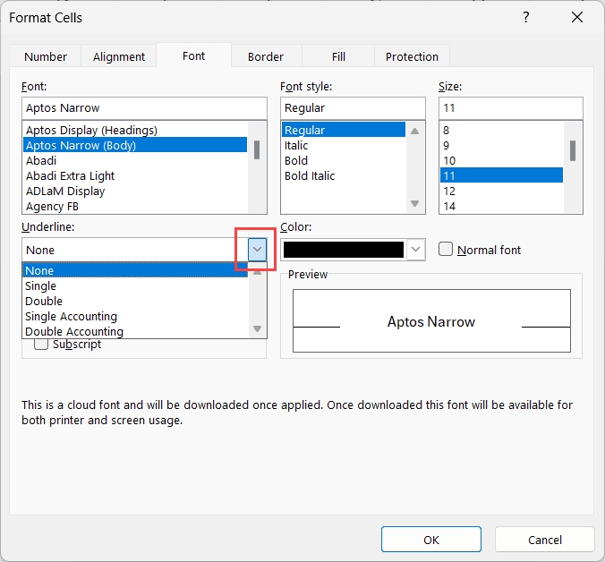
5. Select the Single Accounting or Double Accounting option to apply to the selected cell.

6. Close the Format Cell’s dialog box.

The above steps would apply the Accounting Underline to the selected cells or range of cells.

Now, you must be thinking that the accounting underline and regular underline look the same.

But it’s not the same.

In the next section, I will cover the minor differences between a regular underline and an accounting underline in Excel.

Regular Underline vs. Accounting Underline vs. Bottom Border

The accounting underline format behaves differently with numbers and text.

So, let me show you examples that will make the difference between these three types of underlines clear.

With Numbers

Below is an image that shows the difference between a regular underline, an accounting underline, and the bottom border when used with numbers.

As you would notice, a regular underline is very close to the number, while the accounting underline has a small gap between the number and the line.

The bottom border, on the other hand, would always border the edge of the cell irrespective of the alignment of the content of the cell are

With Text

Below is an image that shows the difference between a regular underline, an accounting underline, and the bottom border when used with text.

When it comes to text, there is a difference between a regular underline and an accounting underline.

With accounting underline, if the cell’s content is a text value, it would underline the entire cell irrespective of the length of the text ring in the cell.

This property of the accounting underline makes it useful in a situation where you don’t want to use borders in the headers but still want to have an underline below the header (as shown below)

In the above example, the accounting order line has been used as a bottom border, but unlike the bottom border, there is a little gap between the lines in the two cells.

How to Remove Underline Formatting in Excel

While you can apply the underline format through the ribbon in the Excel interface, to remove this formatting, you would have to go to the Format Cells dialog box.

Below are the steps to remove the underline format from a cell or range of cells:

1. Select the cells from which you want to remove the underline format
2. Hold the Control key and then press the 1 key to open the Format Cells dialog box, or right-click on the selection and then click on the Format Cells option.
3. In the Format Cells dialog box, click on the Font tab if not selected already.
4. Click on the drop-down below the Underline option and select the None option.
5. Click OK

The above steps would remove the Underline format from the selected cells.

Note: You can also remove the Underline format by clearing the format, But remember that it would remove all the other formatting as well, such as the cell color or the font style

Also read: Excel Custom Number Formatting Tricks

Useful Tips When Using the Underline Formatting in Excel

• Overusing underlining can clutter your spreadsheet and reduce its readability. Use underlining sparingly for maximum impact.
• Underline is one of the formatting options available to you in Excel to highlight cells. You can use it in combination with other options such as bold, italics, or cell color.
• You can use the underline format with Conditional Formatting to dynamically apply it to cells based on their values. Note that within Conditional Formatting, you will only get the regular underline format option and not the accounting underline.
• For underlining multiple cells or entire rows, consider using cell borders instead. It’s often a cleaner solution for larger data sets.

In this article, I showed you how to apply the underline formatting in Excel. I also covered the differences between regular underline format, accounting underline format, and bottom border format.

I hope he found this article helpful. If you have any suggestions or comments for me, do let me know in the comments section.

Other Excel articles you may also like: